Project

Project Overview: Shaping the Future of Math & Data Science

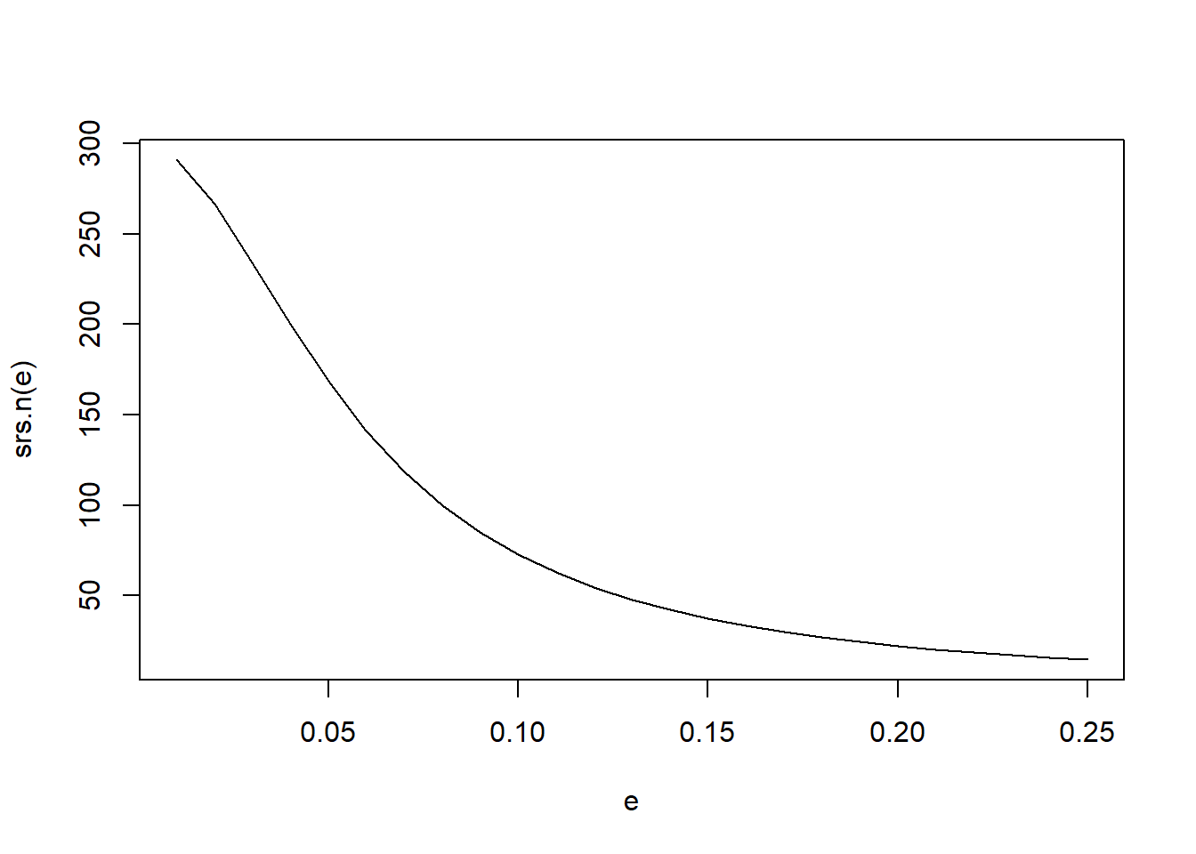
This semester, you will go on a real-world project that will directly impact the future of the Mathematics and Data Science programs at Chico State. Working collaboratively as a class, you will design, implement, and analyze an alumni survey to gather valuable insights about their experiences and career paths. This is your chance to apply the sampling and statistical analysis methods you’ve learned in a practical and meaningful way.

This project isn’t just about crunching numbers; it’s about teamwork, communication, and project management. As a class you will be responsible for:

Defining Roles & Responsibilities: Assign yourselves specific roles within the project (e.g., survey design team, data analysis team, communication lead).
Task Management & Timelines: Establish clear timelines and track progress to ensure successful completion of each project phase.
Stakeholder Communication: Get stakeholder (Math Department faculty, Career center) input in the questions being asked.
Design & Implementing Multiple Sampling Frameworks: Implement multiple sampling methods (e.g., simple random, stratified, cluster) to select representative samples of alumni.
Data Collection & Analysis: Collect survey responses, clean the data, and perform appropriate statistical analyses to answer key research questions. You will also need to compare estimates obtained across the different sampling frameworks to assess their impact on the results.
Final Presentation: Present your findings and recommendations and insights to the Math Department or the assessment committee.

This is a full class collaborative effort, requiring everyone’s active participation and contribution. Every student should take lead on at least one aspect or activity. Your collective efforts will provide valuable data to inform curriculum development, program improvements, and future initiatives within the Mathematics & Statistics departments. Embrace this opportunity to make a real difference!

Milestones

Define Project Goals and Stakeholder Input: Documented agreement on the survey’s objectives and how the results will be used, based on input from stakeholders.
Literature Review and Best Practices Research: Review of existing alumni surveys and research on best practices in survey design and implementation.
Create Sampling Frame: A list of the target population from which the sample will be drawn.
Develop & Test Questionnaire: Draft questionnaire, pilot testing, and revisions based on feedback.
Design Sampling Strategy: Detailed plan for selecting the sample, including justification for the chosen method and sample size calculations.
Collect Data: Completed survey responses. Include metrics on response rate and efforts to address non-response bias.
Data Cleaning: Prepare the data for analysis. Screen for outliers, missing or invalid responses. Create necessary metrics. Create basic tables and summaries for each measures.
Data Analysis: Create analysis plan, conduct analysis and compile results, create visualizations.
Final Presentation: Presentation to stakeholders
Final Report: Comprehensive written report documenting all aspects of the project.

Parameters to be Estimated

Average salary expectations for 1, 2, and 5 years.
Average time taken by alumni to secure their first job
Proportion of alumni who found their degree valuable
Proportion of alumni working in different career sectors
Proportion of alumni who were accepted to or attended graduate school (mathematics oriented) or with a terminal degree
Proportion of alumni who felt they were prepared

Sample Size Determinations

Since most of the parameters to estimate are proportions we will determine the sample size under that framework. Our sampling frame (population size) is $N = 300$ .

We have no prior knowledge of the estimated proportions, so $\hat{p} = \hat{q} = .5$ . We will use this for our estimate of $S$ .
We will set our confidence to be 95%, thus $α = .05$
We will allow our margin of error to vary between 1% and 25%

I created a graph to plot the sample size under an SRS framework using equation 2.30, 2.31 as a function of the margin of error e. We can use this to make a determination of a general total sample size that we will aim for in each of the sampling designs.

srs.n <- function(e){
  n0 <- 1.96^2 / (4*e^2)
  n <- n0 / (1+n0/300)
  return(n)
}
e <- seq(.01, .25, by = .01)
plot(e, srs.n(e), type = "l")

srs.n(seq(.05, .25, by = .05))

[1] 168.45182  72.75023  37.36771  22.23080  14.61766

Sampling Design

Multiple sampling designs were developed as described below.

Read in Sampling frame

library(sampling)
library(tidyverse)

sampling.frame <- googlesheets4::read_sheet(frame.url) |> 
  janitor::clean_names() %>%
  select(fixed_id:assigned_contact_person)

The population size is determined by the size of our sampling frame, and the sample size was determined using the graph above and a class discussion.

N <- NROW(sampling.frame)
n <- 150

SRS

We draw a simple random sample from the entire alumni population without stratifying by any specific variable. Each alumni has an equal probability of being selected, regardless of graduation year, major, or number of majors. This method is easy to implement and ensures that the sample is unbiased with respect to all known and unknown variables. While this approach may not capture differences in key subgroups (e.g., income variation by major or graduation year), it provides a fair and representative overview of the overall alumni population. Since the cost of observation is the same for each unit (zero), SRS is a reasonable choice, particularly when subgroup-specific insights are not the primary goal of the study.

class.seed <- 7+3+5+27+4+510+24+37+42+6+11+64
set.seed(class.seed)
srs.idx <- sampling::srswor(n, N)

srs.sample <- getdata(sampling.frame, srs.idx) %>% 
  select(fixed_id) %>%
  mutate(srs_prob = n/N)

Stratified on Year

In our study we chose to stratify the data to make sure that an alumnus graduation year was accurately represented in the sample. Satisfying typically improves the accuracy and representation of a sample and thus we can accurately account for differences in years. We chose to stratify by year specifically because alumni experiences, job placements, and pay may all depend on how long it has been since they graduated. This is especially important in the past 5-10 years because it would not be surprising if alumni who graduated in or around covid had a much different experience overall than those prior.

We chose to use proportional allocation for our results to more accurately represent the population as a whole. We made the stratum sample sizes proportional to the stratum population sizes. The formula for sample size being $n_{h} = \frac{N_{h}}{N} n$ where $N_{h}$ is the population size of the stratum we are concerned with.

set.seed(class.seed)
strata2.frame <- sampling.frame %>% arrange(expected_grad_year) # sort first

p.1 <- sum(strata2.frame$expected_grad_year==2015)*.5
p.2 <- sum(strata2.frame$expected_grad_year==2016)*.5
p.3 <- sum(strata2.frame$expected_grad_year==2017)*.5
p.4 <- sum(strata2.frame$expected_grad_year==2018)*.5
p.5 <- sum(strata2.frame$expected_grad_year==2019)*.5
p.6 <- sum(strata2.frame$expected_grad_year==2020)*.5
p.7 <- sum(strata2.frame$expected_grad_year==2021)*.5
p.8 <- sum(strata2.frame$expected_grad_year==2022)*.5
p.9 <- sum(strata2.frame$expected_grad_year==2023)*.5
p.10 <-sum(strata2.frame$expected_grad_year==2024)*.5

alloc <- ceiling(c(p.1, p.2,p.3,p.4,p.5,p.6,p.7,p.8,p.9,p.10))

strata.idx <- sampling::strata(data = strata2.frame,      # data set
                 stratanames = "expected_grad_year", 
                 size = alloc,      # stratum sample sizes 
                 method = "srswor")     # method for selecting within strata

Now we extract the unique person identifier (fixed_id) and the sampling probability from the selected sample.

strata.year.sample <- getdata(sampling.frame, strata.idx) %>% 
  select(fixed_id, strata_year_prob = Prob)

Stratified on Major

We hypothesize that students who studied different focuses will be pursuing different types of careers and making different kinds of salaries. Students who double or triple majored will also not have the same experiences as those who share one of their majors. We expect that by stratifying by major, with those with more than one major in a separate stratum, we should be able to expect widely different stratum means for variables like annual income. Since different majors have different course requirements, their feedback on the university will also be different by major. Since we are interested in multiple variables and the observation cost in each stratum will be the same, in this case zero, proportional allocation makes sense as a choice.

First we create a new variable with either a student’s major or if they had multiple majors stored. Will Stratify by this variable

Oops

We have clusters of psych majors b/c their math major was secondary…

sampling.frame$stratamajor <- sampling.frame$major_1
sampling.frame$stratamajor[!is.na(sampling.frame$major_2)] = "Multiple Majors"

sampling.frame.sort.major <- sampling.frame %>% arrange(stratamajor)

Let p be the proportion of total population sampled. We will calculate size of samples drawn from each strata as …. need equations/info here

p <- n/N

strata.size <- table(sampling.frame.sort.major$stratamajor) |> data.frame()
strata.size$n_h <- round(strata.size$Freq * p)

set.seed(class.seed)
strata.major.idx <- sampling::strata(data = sampling.frame.sort.major, 
                              stratanames = "stratamajor", 
                              size = strata.size$n_h, 
                              method = "srswor")

strata.major.sample <- getdata(sampling.frame.sort.major, strata.major.idx) %>% 
  select(fixed_id, strata_major_prob = Prob)

Cluster: Same year same major

need description

One Stage Cluster:

Basic organizing

# renaming to cluster for simplicity
sampling.frame$cluster <- sampling.frame$expected_grad_year

# getting unique cluster ids based on year
(all_clusters <- unique(sampling.frame$cluster))

 [1] 2015 2016 2017 2018 2019 2020 2021 2022 2023 2024

# viewing frequencies of years
(table <- table(sampling.frame$cluster) )


2015 2016 2017 2018 2019 2020 2021 2022 2023 2024 
  29   20   27   32   40   25   29   36   35   25

# picking my sample size, will round to the nearest whole number
weighted.mean(table)

[1] 29.8

NOTE: the number of sampled clusters is based on the average of 30 grads per year to get roughly 150 individuals in the final total sample.

M <- length(unique(sampling.frame$cluster)) # total number of clusters (PSUs, aka GROUPS) in population
m  <- 5 # the number of sampled clusters

Sampling from clusters:

set.seed(class.seed)
# sampling the clusters
(sampled_clusters <- sample(all_clusters, size = m, replace = FALSE))

[1] 2019 2020 2022 2018 2023

# new dataframe of just sampled clusters
cluster.sample <- sampling.frame[sampling.frame$cluster %in% sampled_clusters, c('fixed_id')]

# placeholder for weights
cluster.sample$cluster_prob <- 1

Need to add weights manually since the sampling package was not used.

Create sampling indicators and write back to Google sheets.

Each method will randomly sample a different group of records, there undoubtedly will be substantial overlap. To keep track of which records were chosen in each design, we create separate variables for each design strategy containing the inclusion probability for that specific design. These variables are then added back to the sampling frame in Google Sheets.

sample.these <- sampling.frame %>% 
  select(fixed_id) %>% 
  left_join(srs.sample) %>%
  left_join(strata.major.sample) %>% 
  left_join(strata.year.sample) %>% 
  left_join(cluster.sample) 

head(sample.these)

# A tibble: 6 × 5
  fixed_id srs_prob strata_major_prob strata_year_prob cluster_prob
     <dbl>    <dbl>             <dbl>            <dbl>        <dbl>
1        1    0.503             0.512            0.517           NA
2        2    0.503             0.512           NA               NA
3        3    0.503            NA               NA               NA
4        4    0.503            NA               NA               NA
5        5    0.503             0.505            0.517           NA
6        6    0.503             0.5              0.517           NA

sheets4::range_write(frame.url, 
                     data = sample.these[-1], 
                     range = "Q1:T299", 
                     col_names = TRUE)