library(tidyverse)
agsrs <- read_csv(here::here("data/agsrs.csv"))Ratio and Regression Estimation
Introduction
Motivating Example: Estimating number of people living in France in 1802
In the 1800’s, France did not have a population census count. So some fancy mathematician by the name of Laplace decided he was going to figure it out using sampling and some ideas behind measure of association.
He sampled 30 communities throughout the country, totaling 2,037,615 people.
He reasoned that communities with large populations are also likely to have a large number of registered births. So he looked back in the prior 3 years and counted the number of live births in those communities, finding it to be 215,599. Dividing that number by 3, he calculated this was about 71,866.33 births per year.
He then divided the total number of people, by the number of births pear year, \(\frac{2037615}{71866.33} = 28.352845\), as an estimate of the number of people alive for each new birth.
Assuming this ratio is similar throughout France, he concluded that the total population of France could be estimated by multiplying the total number of annual births in the country by that ratio \(28.352845\).
Laplace was not interested in the number of births on it’s own, but used it as auxilary information to estimate the desired quantity of total population.
Using Auxilary information
Sometimes due to difficulty or cost of data collection, researchers may collect data on secondary measures that are known to be associated with the measure of interest, then leverage that association to improve the precision of the estimators.
Two methods to do this are called Ratio and Regression estimation.
Ratio Estimation in SRS
Let \(y_{i}\) be the measure of interest, and \(x_{i}\) be the auxiliary/secondary/subsidiary variable. Both measurements MUST be taken on the same sample unit \(i\).
Then in a population of size \(N\) the totals for each measure are
\[ t_{y} = \sum_{i=1}^Ny_{i} \qquad t_{x} = \sum_{i=1}^Nx_{i} \]
and their ratio is calculated as \[ B = \frac{t_{y}}{t_{x}} = \frac{\mu_{y}}{\mu_{x}}. \]
Example: Farm yield
Suppose the population consists of agricultural fields of different sizes. Let
- \(y_{i}\) = bushels of grain harvested in field \(i\)
- \(x_{i}\) = acreage of field \(i\).
Then
- \(B\) = average yield in bushels per acre
- \(\mu_{y}\) = average yield in bushels per field
- \(t_{y}\) = total yield in bushels
If we take an SRS, we can then calculate the ratio estimates for these values using
- \(\hat{B} = \frac{\bar{y}}{\bar{x}} = \frac{\hat{t}_y}{\hat{t}_x}\)
- \(\hat{\bar{y}_r} = \hat{B}\mu_x\)
- \(\hat{t}_{yr} = \hat{B}t_x\)
Why use Ratio Estimation
1. It’s our metric of interest
When we sample populations, sometimes we are interested in ratios.
Such as: The average crop yield per acre (Dr.D example) The ratio of liabilities to assets Fish caught per hour Per Capita household income
However, when should/can you use ratio estimation? General rule of thumb, if the denominator of your ratio of interest is something that would be likely to change from sample to sample, ratio estimation is a valid course of action.
Example Let’s say you wanted to find the percent of pages in your favorite magazine that contain at least one advertisement.
To do so, you sample ten different magazine issues. You count the total number of pages in each ith magazine, \(x_i\), and the number of pages that contain at least one advertisement in each ith magazine, \(y_i\).
The proportion of interest, \(\hat{B}\), would be the overall total number of pages with ads, \(\hat{t}_y\), divided by the overall total amount of pages, \(\hat{t}_x\).
Or \(\hat{B} = \frac{\hat{t}_y}{\hat{t}_x}\)
It is important to note that the denominator is not the number of issues you randomly sampled, as that would always be ten, or whatever number of issues you chose to sample. The denominator, in this case, was the sum of pages of the issues you would sample. We want our denominator to be something that could vary, as we would expect it to vary in accordance to whatever the true ratio is.
Common Usages:
Ratio estimation is used every time an SRS is taken to estimate a mean or proportion for a subpopulation
In cluster sampling, ratio estimation is commonly used to estimate means.
2. Unknown N
Sometimes we want to estimate a population total, but the population size N is unknown.
For instance, we want estimate the total number of fish in a haul that are longer than 12 cm.
- First we would take a random sample of fish
- Initially, we would estimate the proportion of fish that are larger than 12 cm, and multiply that proportion by the total number of fish, N. Or, \(\hat{t_y} = N * \bar{y}\)
- However, we cannot do this because we don’t know N
- Find auxiliary information
- We can the fact that having a length of more than 12 cm (y) is related to weight (x).
- Used the proportion of total weight of haul by average weight if the fish. The book explains that its easy to find the total weight of the haul, and the average weight of a fish; AUTHORITY.
- We need to manipulate the following equation:
- \(\frac{\hat{t_y}}{\hat{t_x}} = \frac{\bar{y}}{\bar{x}}\)
- \(\hat{t_y} = \frac{\bar{y}*{\hat{t_x}}}{\bar{x}}\)
- \(\hat{t_y} = \bar{y} * \frac{\hat{t_x}}{\bar{x}}\)
\(\hat{t_y}\): our estimated total number of fish in a haul
\(\bar{y}\): average length of the fish longer than 12 cm
\(\hat{t_x}\): total weight of the haul
\(\bar{x}\): average weight of a fish
Overall, we find an auxiliary information that we can use to relate to another known value. We manipulate the following equation: \(\hat{B} = \frac{\hat{t_y}}{\hat{t_x}} = \frac{\bar{y}}{\bar{x}}\), then add in the known values to find our unknown value.
3. Strong correlation
The higher the correlation coefficient, the better ratio estimation works.
France had no population census in 1802 and Laplace wanted to estimate the number of people living there. Laplace observed the number of births over the next 3 years and came up with the ratio of for every 1 birth there is 28.352845 persons. The number 28 was reached by dividing the total population in the 30 communes by dividing the amount of births over the 3 years by 3. His reasoning was that communes with large, and it would be similar throughout France.
Ratio estimation is often used to increase the precision of estimated means and totals. \(y_{i}\)= numbers of persons in commune i \(x_{i}\)= number of registered births in commune i
Laplace reasoned the ratio estimator would obtain better precision than multiplying the average number of persons by the 30 communes. The larger the population of a commune, the higher the number of registered births, thus the correlation coefficient is likely to be positive.
If the \(t_{x}\)= total number of registered births is known, the mean squared error of the estimated total of the \(\hat{t_y}\) = \(\hat{B_tx}\) is likely to be smaller than the MSE of the population mean and estimator that does not use additional information of registered birth.
4. Adjust for demographic totals
Ratio estimation is used to adjust estimates from the sample to reflect demographic totals.
- Say an SRS was taken of 400 out of 4000 students at a university, and there were 240 women and 160 men in the sample
- Say 84 women and 40 men wanted to be teachers
- Using info from the SRS you’d conclude (4000/400)*(84+40) =1240 students want to be teachers at this university
- If we know there are 2700 women and 1300 men at this university, then we’d conclude (84/240)2700 + (40/160)1300=1270 students want to be teachers
- In this example we used ratio estimation within each gender, so we adjust our estimate for the total according to the ratio within the population
- For this instance, we are adjusting our estimate for the total amount of women who want to be teachers because 60% of the sample is women but the population of women is 67.5%
- \(y_{i}\) = 1 if woman and plans career in teaching, 0 otherwise
- \(x_{i}\) = 1 if woman, 0 otherwise
- (84/240)*2700 = 945 is the ratio estimate for the total amount of women who want to teach
- (40/160)*1300 = 325 is the ratio estimate for the total amount of men who want to teach
- This use of ratio estimation is also called poststratification
5. Ratio Estimation may be used to adjust for non-response.
- Suppose a sample of businesses is taken
- Let \(y_i\) be the amount spent on health insurance by business \(i\) , and let let \(x_i\) be the number of employees in business \(i\) .
- Assume that \(t_x\) the total number of employees in all businesses in the population is known.
We expect that the amount that the business spends on healthcare will be related to the number of employees that the business has. Because some businesses may not respond to the survey, one way to adjust for non-response is:
- Multiply the data \(\bar{y}\) / \(\bar{x}\) using the data from only the respondents by the population total \(t_x\).
If companies with fewer employees are less likely to respond, and \(y_i\) is proportional to \(x_i\), then we would expect the estimate \(N\bar{y}\) to overestimate the population total \(t_y\)
But, in the ratio estimation, the estimate is likely to be smaller than N because companies with many employees are more likely to respond.
Therefore, the ratio estimate will help compensate for the non-response of small companies.
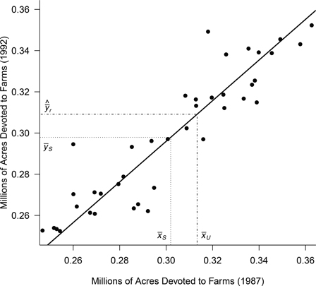
Example: Total acreage of farms in 1992, based on data from ’87.
Pretend it’s 1992 and since we did a census of farmland in 1987 we the true population values. But that was super expensive so we want to find a better way for this year.
In 1987 a total of \(t_x\) = 964,470,625 acres were devoted to farms across the 3,078 counties in the US, with average acres per county \(\mu_x\) = 313,343.3. Use these values along with data taken from an SRS (agsrs.csv) to estimate the total and average number acres devoted to farmland in 1992.
Calculate the correlation coefficient, and create a scatterplot of
acres87againstacres92first to assess the linear correlation between these two measures and to comment on if it’s even reasonable to use 1987 values to estimate 1992 amounts.Use the population values from 1987 along with the data in the variable
acres92to calculate \(\hat{B}, \hat{\bar{y}}_r\), and \(\hat{t}_{yr}\) for 1992.Compare \(\hat{t}_{yr}\) to \(\hat{t}_{srs}\) for 1992.
- Visualize the relationship between acres in 1987 and 1992 on the SRS of \(n=300\). It is important to use both a linear model straight line, and the lowess smoother line to assess how well a linear model may fit this relationship.
ggplot(agsrs, aes(x=acres87, y=acres92)) + geom_point() +
  geom_smooth(method="lm", col="red", se=FALSE) +
  geom_smooth(col="blue", se=FALSE) + theme_minimal()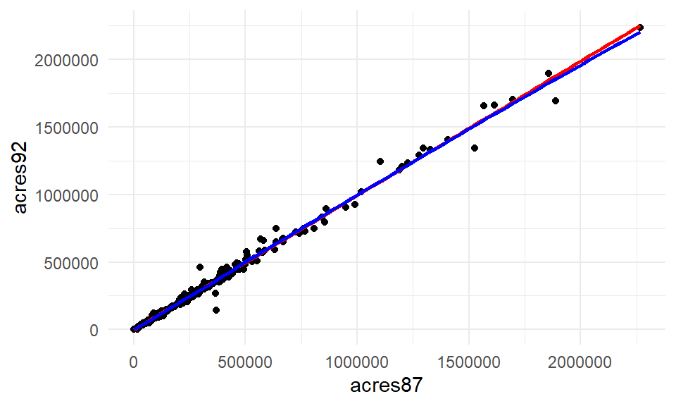
cor(agsrs$acres87, agsrs$acres92)[1] 0.995806The blue and red lines are nearly overlapping, and the correlation coefficient is incredibly high at 0.996. A linear model fits this relationship well, and so the ratio estimate is reasonable to use.
- Calculate estimated ratio and estimators for average and total acrage.
Estimated Ratio \(\hat{B} = \frac{\bar{y}}{\bar{x}}\)
x.bar <- mean(agsrs$acres87)
y.bar <- mean(agsrs$acres92)
(B.hat = y.bar/x.bar)
[1] 0.9865652Ratio Estimator for \(\hat{\bar{y}}_r = \hat{B}\mu_x\)
B.hat * 313343.3[1] 309133.6Ratio Estimator for \(\hat{t}_{yr} = \hat{B}t_x\)
B.hat * 964470625[1] 951513191- Compare the ratio estimator of the total to the estimate obtained under SRS
y.bar*3078[1] 916927110In this case, the ratio estimator is smaller than the estimate obtained from the SRS directly. Let’s see why this may be the case.
- We notice that \(\bar{x} \lt \mu_x\), so our SRS underestimates the true population mean from 1987.
- Since \(x\) and \(y\) are positively correlated, it is reasonable to expect that \(\bar{y}\) will similarily underestimate \(\mu_y\)
- However, the ratio estimator \(\hat{\bar{y}}_r\) gives a more precise estimate of \(\mu_y\) because \(\bar{y}\) is multiplied by the factor \(\frac{\mu}{\bar{x}}\), which corrects for that underestimation.
Regression Estimation in SRS
Regression estimation uses the method of ordinary least squares to calculate estimates for the slope \(B_1\) and intercept \(B_{0}\) of a ‘line of best fit’ between the outcome measure of interest \(y\) and the auxiliary variable \(x\).
\[ y = B_0 + B_1x \]
where
\[ \hat{B}_1 = \frac{rs_y}{s_x} \qquad \hat{B}_0 = \bar{y} - \hat{B}_1\bar{x} \]
where \(r\) is the sample correlation coefficient between \(x\) and \(y\), and \(s_x\) and \(s_y\) are sample standard deviations of \(x\) and \(y\) respectively.
Regression estimation uses the sample correlation between \(y\) and \(x\) to obtain an estimate for \(\mu_y\) with increased precision.
Example: Dead trees
Instead of wandering around the forest looking for dead trees and getting bitten by spiders, we can take pictures of an area and then count the dead trees in the photographs. While this can be quicker, there is a chance of misclassification (identifying a live tree as dead, or a dead tree as living) or not seeing trees altogether.
So let’s divide the area into 100 square plots, take pictures of all 100, then take an SRS of 25 plots for in person counting. Then we’ll use regression estimation to estimate the actual average number of dead trees in a plot, using the estimates counted from the photos.
First read in the data and take a glimpse of the values.
library(tidyverse)
trees <- read_csv(here::here("data/deadtrees.csv"))
glimpse(trees)
Rows: 25
Columns: 2
$ photo <dbl> 10, 12, 7, 13, 13, 6, 17, 16, 15, 10, 14, 12, 10, 5, 12, 10, 10,…
$ field <dbl> 15, 14, 9, 14, 8, 5, 18, 15, 13, 15, 11, 15, 12, 8, 13, 9, 11, 1…The variable photo is our auxiliary variable \(x\), containing the count of dead trees from the photograph in each of the sampled plots. The variable field is the outcome variable \(y\), the count of dead trees from field observation.
To visualize this relationship, we create a scatterplot of photo against field, and adding a best fit line using the method=lm argument to geom_smooth().
ggplot(trees, aes(x=photo, y=field)) +
  geom_point() + geom_smooth(method="lm", se=FALSE)
The equation of that line can be found using the lm function.
lm(field ~ photo, data=trees)
Call:
lm(formula = field ~ photo, data = trees)

Coefficients:
(Intercept)        photo
     5.0593       0.6133
\[ \hat{y} = 5.06 + 0.613x \]
The average number of dead trees per plot from the photo count is \(\mu_x = 11.3\), so we can plug this value into \(x\) and get our estimated \(\hat{y}_{reg}\)
5.06 + 0.613*11.3[1] 11.9869On average, we estimate there to be 11.986 dead trees per plot.
Estimation using R
The above examples were from SRS’s, and we know that sampling methods can get more complex, and that we typically need to adjust for weights. So we look now at how to use the survey package functions to calculate ratio and regression estimates.
library(survey)Ratio est using svyratio
The svyratio function is what we’ll use to calculate ratio estimates using survey data. For this example we’ll use the farmland example where we’re predicting the total number of acres devoted to farming in 1992, based on that same value in 1987.
- Add the survey weights and population size \(N\) (for the fpc) to the data set if not already present.
agsrs$N <- 3078
agsrs$wt <- 3078/300 #N/n- Set our survey design
ag.design <- svydesign(id = ~1, # no clustering
                        weight = ~wt,
                        fpc = ~N, # pop size to be used in FPC
data = agsrs)- estimate the ratio \(\hat{B}\) as
acres92/acres87.
(b.hat <- svyratio(numerator = ~acres92,
                   denominator = ~acres87,
                   design = ag.design))
Ratio estimator: svyratio.survey.design2(numerator = ~acres92, denominator = ~acres87,
design = ag.design)
Ratios=
acres87
acres92 0.9865652
SEs=
acres87
acres92 0.005750473- Use this model to predict \(t_{r, acres in 1992}\), the ratio estimate for the total number of acres in 1992.
# provide the population total of x
xpoptotal <- 964470625
# Ratio estimate of population total
predict(b.hat, total=xpoptotal)
$total
acres87
acres92 951513191
$se
acres87
acres92 5546162Regression est using svyglm
The svyglm function calculates regression coefficients from survey data. It is the analog of the R function glm which fits generalized linear models.
- Add the survey weights and population size \(N\) (for the fpc) to the data set if not already present.
trees$wt <- 4
trees$N <- 100- Set our survey design
dtree <- svydesign(id = ~1, # no clustering
                   weight = ~wt,
                   fpc = ~N, # pop size to be used in FPC
data = trees)- Fit the regression model and estimate the slope and intercept coefficients.
tree.model <- svyglm(field~photo, design = dtree)
coef(tree.model) # print the coefficients
(Intercept) photo
5.0592920 0.6132743 - Use this model to predict \(\hat{\bar{y}}\) using \(\mu_x = 11.3\)
We create a new data frame that only contains the value for the \(x\) variable we want to predict. The variable name in newdata has to match the one in the tree.model. This new data then is passed into the predict function.
newdata <- data.frame(photo = 11.3)
predict(tree.model, newdata)
link SE
1 11.989 0.418predict(tree.model, newdata, df = degf(tree.model)) %>% confint() 2.5 % 97.5 %
1 11.16998 12.8086We can be 95% confident that there are on average 12.0 (95% CI 11.2-12.8) dead trees per plot in the 100 plot area under investigation.