Stratified Sampling

A method to use additional information about the population in the survey design. Lohr Ch 3.

Author

DRAFT - 458 class

Published

March 20, 2023

library(here); library(tidyverse);library(knitr)
library(sampling); library(survey)

What is Stratified Sampling

Overview

A sampling technique in which we divide the desired population into subgroups called strata
Each individual is necessarily in a single strata; no overlap within strata
All strata consist of the entire population
An SRS is taken from each strata, then results can be pooled to make inferences about the entire population

Why Use A Stratified Sample?

Protection from bad samples; less likely of drawing a non representative sample through pure chance
Want data of known subgroups (i.e., if we are interested in people’s heights, we know that men tend to be taller than women)
Convenience / cost effectiveness – At what point will this compromise the legitimacy of the study?
Lowers variance when done properly; variance within each strata is likely lower than the population variance
you do not have to sample the same fraction of observations in each stratum. If the variability is higher in a certain strata then you can try to reduce the variability of the estimated total by taking more observations from that stratum.

Motivating Example - Estimating the average number of farm acres.

agpop <- read_csv(here("data", "agpop.csv"))

In Example 2.6 we took a SRS to find the average number of farm acres per county. Even though our methods of taking an SRS were correct, some areas of the country were over or underrepresented due to the variability in the size of farms in different regions in the country. An example of this would be that western states in the U.S tend to be larger, and therefore tend to have larger farms.

To try and fix this, we can use a stratified sample can give balance to the sample on the stratifying variable, which in this case would be region that the farms are located.

To begin, we can divide our data into four regions (these are the strata):

unique(agpop$region) # the four regions and their names

[1] "W"  "S"  "NE" "NC"

Previously we sampled 10% of the population with an SRS, and so to be able to compare our results with our stratified sample, we should sample 10% of the population from each strata through four separate and independent SRS’s.

The process to do this would be to take the four regions, number off the counties that are in the region, calculate what number of counties is 10% of the total number of counties in the region, and select that many numbers from the list of numbered counties.

Details on how to do this in R is covered in a later section. For now we will use the agstrat dataset from the book as the stratified sample.

agstrat <- read_csv(here("data", "agstrat.csv"))

Exploring the distribution of farm acreage in 1992 by region.

boxplot(acres92/10^6 ~ region, data = agstrat,
        xlab = "Region", ylab = "Millions of Acres")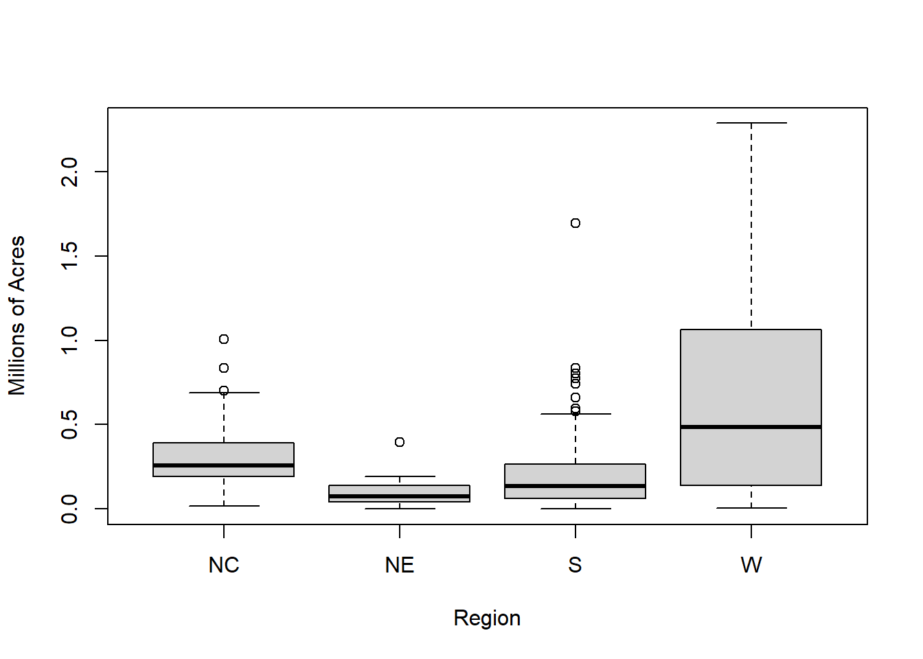

The thick line for each region is the median of the sample data from that region. The upper and lower horizontal lines of the boxes are the 25th and 75th percentiles.

The Northeast has the lowest median and the smallest variance. The West has the highest median and the highest mean and variance. The distribution of farm acreage appears to to be positively skewed in each region.

The summary statistics \(\bar{y}_{h}\) and \(s^{2}_{h}\) can be calculated using R after grouping by the stratification variable.

table3.1 <- agstrat %>% 
   group_by(region) %>% 
   summarize(y.bar.h = mean(acres92),
             s2.h    = var(acres92),
             n.h     = n())

counties_in_pop <- table(agpop$region)
new_table3.1 <- cbind(table3.1, counties_in_pop)
new_table3.1 <- select(new_table3.1, -Var1) # drop the extra variable 
colnames(new_table3.1) <- c("Region", "Sample Avg in Region", "Sample Variance in Region", 
"Number of Counties in Region", "Number of Counties in Population")

kable(new_table3.1)

Region	Sample Avg in Region	Sample Variance in Region	Number of Counties in Region	Number of Counties in Population
NC	300504.16	29618183543	103	1054
NE	97629.81	7647472708	21	220
S	211315.04	53587487856	135	1382
W	662295.51	396185950266	41	422

Lohr Table 3.1. Summary statistics for each stratum

These summary statistics can be used to calculate estimates of the total number of farms acres, and estimated variance of the total within each of the four stratum (Table 3.2 below)

Because we took an SRS in each stratum, we can use the following equations to estimate population quantities for each stratum.

\(\hat{\tau_{h}} = N * \bar{y}_{h} \quad \mbox{ and } \quad \hat{V}(\hat{\tau}_{h}) = N_{h}^{2} * \hat{V}(\bar{y}_{h})\)

We can estimate the total number of acres devoted to farming in the United States in 1992 by summing the estimated totals for each stratum.
The variance of the total is the sum of the variances of the estimated stratum totals.

More information on how to do this in the next section.

⭐ You try it.

Explore the distribution of farm acreage in 1987 by region. Create a table of summary statistics and a boxplot. Discuss your findings.

Solution

agstrat %>%
  group_by(region) %>%
  summarize(y.bar = mean(farms87),
            s2 = var(farms87),
            n. =n())

# A tibble: 4 × 4
  region y.bar      s2    n.
  <chr>  <dbl>   <dbl> <int>
1 NC      837. 156050.   103
2 NE      605. 175660.    21
3 S       610. 231169.   135
4 W       615. 275507.    41

ggplot(agstrat, aes(x = region, y = farms87, fill = region)) +
  geom_boxplot() +
  labs(title = "Box Plot of Farm acreage in 1987 by Region",
       x = "Region",
       y = "Acreage")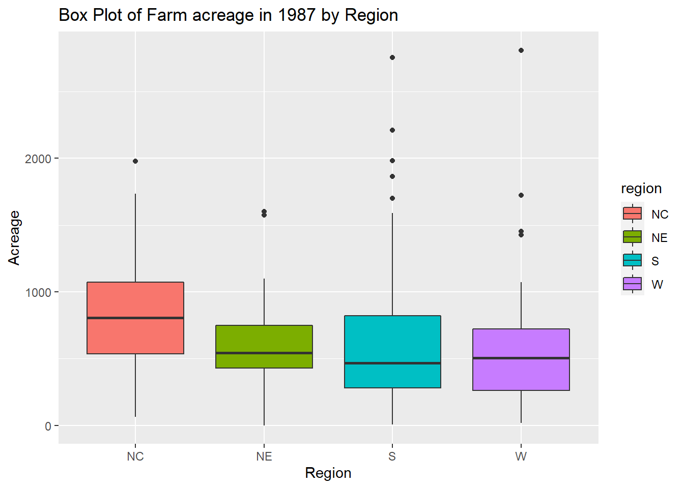

Both the boxplot and the table suggest that, on average, farms in the north-central region have the most acreage (837 acres). The mean acreages in the North East, South, and West regions are similar, ranging from 605-615 acres. The variances for all four regions are large, suggesting the individual acreage of the farms varies greatly and is not precise. The results indicate that the quantity’s mean value for area North Central is 837.0485 with a variance of 156503.3 and a sample size of 103. The mean value for area North East is 605.2381, with a variance of 175660.4 and a sample size of 21. With a sample size of 135 and a variance of 231169.2, the mean value for region South is 610.4889. For region West with a sample size of 41, the mean value is 614.7073 with a variance of 275506.9.

Gain from stratification

Observations within strata are more similar to each other, than they are to the population as a whole
reduction in variance in individual strata can lead to a reduced variance for the population estimate.

Definition: Relative gain from stratification

\[ \frac{\hat{Var_{strata}}}{\hat{Var_{SRS}}} \]

From the Farm example, this ratio was calculated to be 0.75. That means we would only need 0.75*300 = 225 observations from a stratified sample to obtain the same precision as from a SRS of 300.

By sampling within strata, we are “borrowing” information from other similar observations.

Clean up

rm(counties_in_pop, table3.1, new_table3.1)

Theory of Stratified Sampling

Notation and Formulas used in Stratified Random Sampling

To take a stratified random sample, we take a SRS from each stratum, so that \(n_h\) units are sampled from the \(N_h\) population units in stratum \(h\).
Statistics and sample sizes for stratum \(h\) have subscript \(h\) where \(h=1 \ldots H\) index strata
When a statistic has the subscript \(str\), that means that the statistic is the combined estimate across all stratas.
- \(\bar{y}_{str}\) is a weighted average of the sample stratum means
- \(\hat{p}_{str}\) estimated proportion of population units having a specified characteristic. Recall a proportion is a mean of a variable that takes on the values 0 and 1.
\(y_{hj}\) value of the \(j\)th unit in strata \(h\)
\(\sum_{j=1}^{n_{h}}\) means to sum of all units in strata \(h\)
\(\sum_{j}\) means to sum over the units that were sampled from in strata \(h\)
\(\sum_{h}\) is shorthand for \(\sum_{H=1}^{h}\)

Formulas
Explanations

Measure	Population \((\theta)\)	Sample \((\hat{\theta})\)
Sample size in strata \(h\)	\(N_{h}\)	\(n_{h}\)
Overall sample size	\(N = \sum^{H}_{h=1} N_{h}\)	\(n = \sum^{H}_{h=1} n_{h}\)
Var(y) in strata \(h\)	\(\sigma_{h}^2 = \frac{1}{N_{h}-1}\sum_{j=1}^{N_{h}}(y_{hj}-\mu_{h})^2\)	\(s_{h}^2 = \frac{1}{n_{h}-1}\sum_{j}(y_{hj}-\bar{y}_{h})^2\)
Total in strata \(h\)	\(\tau_{h} = \sum_{j=1}^{N_{h}} y_{hj}\)	\(\hat{\tau}_{h} = N_{h}\bar{y_h}\)
Overall total	\(\tau = \sum_{h=1}^{H} \tau_{h}\)	\(\hat{\tau}_{str} = \sum_{h=1}^{H}N_{h}\bar{y}_{h}\)
Mean in strata \(h\)	\(\mu_{h} = \frac{\tau_{h}}{N_{h}}\)	\(\bar{y}_{h} = \frac{1}{n_{h}}\sum_{j} y_{hj}\)
Overall mean	\(\mu = \frac{\tau}{N}\)	\(\bar{y}_{str} = \sum_{h=1}^{H} \frac{N_{h}}{N}\bar{y}_{h}\)
Proportion in strata \(h\)	\(p_{h} = \mu_h\)	\(\bar{y}_h = \hat{p}_h\)
Variance of \(p_{h}\)	\(\sigma_h^2=\frac{N_h}{N_h-1} p_h(1-p_h)\)	\(s_h^2=\frac{n_h}{n_h-1} \hat{p}_h(1-\hat{p}_h)\)
Overall proportion	\(p_{str} = \sum_{h=1}^{H} \frac{N_h}{N} p_h\)	\(\hat{p}_{str} = \sum_{h=1}^{H} \frac{N_h}{N}\hat{p}_h\)

Measure	Population \((\theta)\)	Sample \((\hat{\theta})\)
Sample size in strata \(h\)	number of population units in stratum h	sample size taken in stratum h
Overall sample size	total population size, from all strata	total sample size, from all strata
Total in strata \(h\)	population total in strata h	estimated population total in stratum h
Overall total	population total	estimated population total
Mean in strata \(h\)	population mean in strata h	sample mean in stratum h
Overall mean	population mean	weighted average of the sample stratum means
Variance of the mean	population variance in stratum h	sample variance in stratum h
Proportion in strata \(h\)
Variance of proportion
Overall proportion

With estimated variances;

Within strata total \(\hat{V}(\hat{\tau}_{h}) = (1-\frac{n_h}{N_h})N^2 \frac{s^2_h}{n_h}\)
Within strata mean \(\hat{V}(\bar{y}_{h}) = \frac{1}{N^2}V(\hat{\tau}_{h})\)
Overall population total \(\hat{V}(\hat{\tau}_{str}) = \sum_{h=1}^H (1-\frac{n_h}{N_h})N^2 \frac{s^2_h}{n_h}\)
Population proportion \(\hat{V}(\hat{p}_{str}) = \sum_{h=1}^H (1-\frac{n_h}{N_h}) (\frac{N_h}{N})^2 \frac{\hat{p}_h (1-\hat{p}_h)}{n_h-1}\)
Estimated total number of population units having a specified characteristic: \(\hat{t}_{\it{str}} = \sum_{h=1}^H N_h \hat{p}_h\)

Confidence Interval for Stratified Random Sample

If either the sample sizes within each stratum are large or the sampling design has a large number of strata, then the confidence interval for the population mean \(\bar{y}\mu\) is:

\[ \bar{y}_{str}= \pm z_{\alpha /2 } SE (\bar{y}_{str})\]

However, most survey packages use a \(t_{n-H}\) distribution instead of using the normal assumption.

Example: Estimate the total number of farm acres in 1992 (Table 3.2)

The best way to understand an equation, is to try to use it in a calculation.

Calculate summary statistics for each region. This was seen earlier as new_table3.1

strata.summary.stats <- agstrat %>% 
   group_by(region) %>% 
   summarize(y.bar.h = mean(acres92),
             s2.h    = var(acres92),
             n.h     = n())

Calculate Population region sizes, add this vector to the data frame created above.

(region.size <- agpop %>% group_by(region) %>% tally())

# A tibble: 4 × 2
  region     n
  <chr>  <int>
1 NC      1054
2 NE       220
3 S       1382
4 W        422

strata.summary.stats$N.h <- region.size$n
strata.summary.stats

# A tibble: 4 × 5
  region y.bar.h          s2.h   n.h   N.h
  <chr>    <dbl>         <dbl> <int> <int>
1 NC     300504.  29618183543.   103  1054
2 NE      97630.   7647472708.    21   220
3 S      211315.  53587487856.   135  1382
4 W      662296. 396185950266.    41   422

Calculate the sample total \(\hat{\tau}_{h} = N_{h}\bar{y_h}\).

strata.summary.stats$tau.hat.h <- strata.summary.stats$y.bar.h * strata.summary.stats$N.h
strata.summary.stats

# A tibble: 4 × 6
  region y.bar.h          s2.h   n.h   N.h  tau.hat.h
  <chr>    <dbl>         <dbl> <int> <int>      <dbl>
1 NC     300504.  29618183543.   103  1054 316731380.
2 NE      97630.   7647472708.    21   220  21478558.
3 S      211315.  53587487856.   135  1382 292037391.
4 W      662296. 396185950266.    41   422 279488706.

Calculate the within-strata variance of this total \(\Big(1 - \frac{n_{h}}{N_{h}}\Big)N^{2}_{h}\frac{s^{2}_{h}}{n_{h}}\).

strata.summary.stats <- strata.summary.stats %>%
  mutate(var.tau.hat.h = 
           (1 - n.h/N.h)*(N.h^2)*(s2.h/n.h)
  )
strata.summary.stats

# A tibble: 4 × 7
  region y.bar.h          s2.h   n.h   N.h  tau.hat.h var.tau.hat.h
  <chr>    <dbl>         <dbl> <int> <int>      <dbl>         <dbl>
1 NC     300504.  29618183543.   103  1054 316731380.       2.88e14
2 NE      97630.   7647472708.    21   220  21478558.       1.59e13
3 S      211315.  53587487856.   135  1382 292037391.       6.84e14
4 W      662296. 396185950266.    41   422 279488706.       1.55e15

Calculate the overall total \(\hat{\tau}_{str}\) and variance \(\hat{V}\big(\hat{\tau}_{str}\big)\) by summing these values across the strata.

(tau.hat.str <- sum(strata.summary.stats$tau.hat.h))

[1] 909736035

(V.tau.hat.str <- sum(strata.summary.stats$var.tau.hat.h))

[1] 2.541899e+15

The estimated total number of acres devoted to farming is 909,736,035, with standard error 50,417,248. These numbers match those found in Table 3.2.

⭐ You try it

Siniff and Skoog (1964) used stratified random sampling to estimate the size of a herd of Alaskan caribou in 1992. Using prior known caribou density estimates for the region, the researches divided the area into 6 strata, then within each strata they formed a grid where each cell was 4 sq miles. They then randomly sampled the grids within each strata. The summary information from each strata is contained in the table below.

Stratum	N.h	n.h	y.bar.h	s2.h
A	400	8	24.1	5575
B	30	10	25.6	4064
C	61	37	267.6	347556
D	18	6	179.0	22798
E	70	39	293.7	123578
F	120	21	33.2	9795

Use this information and the equations from this chapter to calculate the estimated total number of caribou in this region in Alaska with a 95% CI.

Solution

# Create data frame
caribou <- data.frame(
  Stratum = c("A", "B", "C", "D", "E", "F"), 
  N.h = c(400, 30, 61, 18, 70, 120), 
  n.h = c(98, 10, 37, 6, 39, 21), 
  y.bar.h = c(24.1, 25.6, 267.6, 179, 293.7, 33.2), 
  s2.h = c(5575, 4064, 347556, 22798, 123578, 9795))

# within strata total
caribou$tau.hat.h <- caribou$y.bar.h *caribou$N.h

# within strata variance
caribou <- caribou %>%
  mutate(var.tau.hat.h = (1 - n.h/N.h)*(N.h^2)*(s2.h/n.h)
  )

# overall total and variance of the total
(tau.hat.str <- sum(caribou$tau.hat.h))

[1] 54496.6

V.tau.hat.str <- sum(caribou$var.tau.hat.h)

# calculating at CI using a t_{n-H} distribution
n.caribou <- sum(caribou$n.h)
n.strata <- length(caribou$Stratum)
df <- n.caribou - n.strata

(crit.value <- qt(.975, df))

[1] 1.971603

s.error <- sqrt(var.tau.hat.str)

Error in eval(expr, envir, enclos): object 'var.tau.hat.str' not found

(tau.hat.str - crit.value*s.error)

Error in eval(expr, envir, enclos): object 's.error' not found

(tau.hat.str + crit.value*s.error)

Error in eval(expr, envir, enclos): object 's.error' not found

missing

CI and interpretation of CI

This CI only explains uncertainty due to sampling error, if researchers tend to miss animals, this CI will be low.

⭐ You try it

The ACLS intends to use a stratified random sample to study publications and library use among members. They divide their data into discipline, making 7 stratas.

Use the summary table below to estimate the the percentage and number of respondents that are female in those seven disciplines.

Membership	Valid.Returns	Female.members
9100	636	0.38
1950	451	0.27
5500	481	0.18
10850	611	0.19
2100	493	0.36
5500	575	0.13
9000	588	0.26

Solution

First extract the table information into vectors.

Nh <- c(9100,1950,5500,10850,2100,5500,9000)
nh <- c(636,451,481,611,493,575,588)
ph <- c(.38,.27,.18,.19,.36,.13,.26)
N <- sum(Nh)

Then the overall estimated proportion of female members in the societies is calculated as

(p.str = sum((Nh/N)*ph))

[1] 0.2465227

with variance

sum((1-(nh/Nh))*((Nh/N)^2)*((ph*(1-ph))/(nh-1)))

[1] 5.067478e-05

The total number of female members in this society is calculated as

N*p.str

[1] 10847

There are an estimated 10,847 female members.

Clean up

rm(list=ls()[!ls() %in% c("agpop", "agstrat","caribou")])

Sampling Weights

How are weights calculated?

Sampling weights in the context of Stratified Sampling function almost identically as they did in SRS.

For any unit \(j\) in a stratum \(h\), a sampling weight(\(w_{hj}\)) is still the inverse of an inclusion probability(\(\pi_{hj}\)). However, because the population of a stratum, \(N_h\), and the size of a sample of a stratum, \(n_h\), don’t have to be constant within a population of \(H\) strata, each stratum will have different sampling weights.

\(w_{hj}= \frac{1}{\pi_{hj}}=\frac{N_h}{n_h}\)

How are weights used?

The weights are directly applied to the values of \(y\) before being used in any calculations.

\[\hat{t}_{str}= \sum_{h=1}^H\sum_{j\in S_h} w_{hj}y_{hj}\]

is the estimator of the total population using a stratified sample, and

\[\bar{y}_{str}= \frac{\hat{t}_{str}}{\sum_{h=1}^H\sum_{j\in S_h} w_{hj}}= \frac{\sum_{h=1}^H\sum_{j\in S_h} w_{hj}y_{hj}}{\sum_{h=1}^H\sum_{j\in S_h} w_{hj}}\]

is the estimate for a population mean using stratified sampling.

Example: Re-Estimate the total number of farm acres in 1992 using sample weights

Note, this agriculture example was designed so that each county in the US had approximately the same probability of appearing in the sample.

Calculate stratum weights. Sometimes this is given to you, othertimes you have to calculate it.

strat.weights <- data.frame(
  region = table(agpop$region) %>% names(),
  N.h = table(agpop$region) %>% as.vector(), 
  n.h = table(agstrat$region) %>% as.vector()
)
strat.weights$wt <- strat.weights$N.h / strat.weights$n.h
strat.weights

  region  N.h n.h       wt
1     NC 1054 103 10.23301
2     NE  220  21 10.47619
3      S 1382 135 10.23704
4      W  422  41 10.29268

Merge those weights back onto the sample data, joining by region.

agstrat <- agstrat %>% left_join(strat.weights)
table(agstrat$wt)


10.2330097087379  10.237037037037 10.2926829268293 10.4761904761905 
             103              135               41               21

This last table is used to confirm that the number of weighting values equals the strata sample sizes.

Calculate the weighted values \(w_{hj}y_{hj}\). The weights need to be applied to the individual data points, \(y_{jh}\), then all the above calculations can occur again.

agstrat$wtd.acres92 <- agstrat$acres92 * agstrat$wt

Calculate the weighted totals and variances within strata. Include the population and sample sizes within each strata in the group_by statement so it can remain on the grouped dataset for later use.

(wt.str.sum.stats <- agstrat %>%
   group_by(region, N.h, n.h) %>% 
   summarize(y.bar.h = sum(wtd.acres92)/n.h,  
             s2.h    = (1/(n.h-1))*sum((wtd.acres92-y.bar.h)^2)
             ) %>%
   unique() # this removes duplicate rows created in the variance function
 )

# A tibble: 4 × 5
# Groups:   region, N.h, n.h [4]
  region   N.h   n.h  y.bar.h    s2.h
  <chr>  <int> <int>    <dbl>   <dbl>
1 NC      1054   103 3075062. 3.10e12
2 NE       220    21 1022788. 8.39e11
3 S       1382   135 2163240. 5.62e12
4 W        422    41 6816798. 4.20e13

Calculate within strata totals and variances \(\hat{\tau}_{h}\) and \(\hat{V}(\hat{\tau}_{h})\).

(wt.str.sum.stats <- wt.str.sum.stats %>% 
    mutate(tau.hat.h = y.bar.h * N.h , 
           var.tau.hat.h = (1 - n.h/N.h)*(N.h^2)*(s2.h/n.h)))

# A tibble: 4 × 7
# Groups:   region, N.h, n.h [4]
  region   N.h   n.h  y.bar.h    s2.h   tau.hat.h var.tau.hat.h
  <chr>  <int> <int>    <dbl>   <dbl>       <dbl>         <dbl>
1 NC      1054   103 3075062. 3.10e12 3241115284.       3.02e16
2 NE       220    21 1022788. 8.39e11  225013466.       1.75e15
3 S       1382   135 2163240. 5.62e12 2989597592.       7.17e16
4 W        422    41 6816798. 4.20e13 2876688634.       1.65e17

Calculate the overall total \(\hat{\tau}_{str}\) and variance \(\hat{V}\big(\hat{\tau}_{str}\big)\) by summing these values across the strata.

(tau.hat.str <- sum(wt.str.sum.stats$tau.hat.h))

[1] 9332414976

(V.tau.hat.str <- sum(wt.str.sum.stats$var.tau.hat.h))

[1] 2.682133e+17

Note. This value for tau.hat.str does not match what the book says. Not sure where the error is at.

⭐ You try it Caribou weights

In the caribou example, strata A had N=400 and n=98, so the sampling weight is 400/98 or 4.08.

caribou$w.hj <- caribou$N.h/ caribou$n.h
caribou %>% select(Stratum:n.h, w.hj)

  Stratum N.h n.h     w.hj
1       A 400  98 4.081633
2       B  30  10 3.000000
3       C  61  37 1.648649
4       D  18   6 3.000000
5       E  70  39 1.794872
6       F 120  21 5.714286

Note: We cannot re-estimate the total number of caribou using the information provided because we are given the summary statistics \(\bar{Y}_h\), not the raw data \(y_{hj}\). To re-estimate the total number of caribou we would need to multiply the weights \(w_{h}\) to \(y_{hj}\).

Clean up

rm(list=ls()[!ls() %in% c("agpop", "agstrat","caribou")])

Allocation Methods

Designing the survey is the most important part of using a survey in research. If the survey is badly designed, then no amount of analysis will yield the needed information.

Simple random sample was easy - you just need to figure out the end sample size. For stratified sampling, we need to define the strata, and the sample size within each strata.

Method 1: Proportional Allocation

The number of sampling unit in a stratum is proportional to the population of each stratum.

Probability selection (n/N) the same for each stratum (n being the number of sampling units in the stratum and N being the population of the stratum)
Weight of each sample will be the same
Stratified sampling estimate of the population mean is the average of all observations
Self-weighting: every unit in sample carries the same weight
When the strata are large enough, \(Var(\bar{y}_{str})\) will almost always be less than the population variance of \(Var(\bar{y}_{srs})\) of the same sample size
The more the means of the strata differ, the more precision you will gain from using proportional allocation.
When the variances are roughly the same across all strata, proportional allocation is likely your best bet for increasing precision

Method 2: Optimal Allocation

Allocation of sampling units to strata so that the variance of the estimator is minimized for a given total cost.

It is best to use when the sampling units are from corporations, cities, hospitals, or wherever the size varies largely. You want to get the most from the least cost.
- E.g. If we wanted to estimate trade with Europe, the variance among large corporations would be larger than when compared to small corporations, so we’d sample more large corporations
When the variances of the strata are significantly different, optimal allocation lowers the cost
When certain strata are more expensive to sample than others, optimal allocation may be useful
Generally, heavily sample from a stratum if:
- Stratum is large
- Variance of stratum is large
- Its cheap

Optimization methods:

Disproportional allocation: Allocation of sampling units to strata so that the sampling fractions \(\frac{n_h}{N_h}\) are unequal
Oversampling: Selecting more observations in a stratum than would be called for in proportional allocation. An oversampled stratum has \(\frac{n_h}{N_h} \gt \frac{n}{N}\)
Neyman Allocation: special case of optimal allocation where the costs in the strata are about equal, but the variances are not
- If variances within strata are specified correctly, Neyman Allocation will give a smaller variance than proportional allocation

Method 3: Allocation for Specified Precision within Strata

Sometimes we are less interested in estimating the overall population values, and more interested in comparing the totals or means across stratum

In this case we would need to determine the sample size for each stratum that corresponds to a specific level of precision.

Which allocation to use?

Proportional Allocation

should be used when you want your sample to be a mini version of the population.
the only knowledge about your data that is needed is N, making this a better option for some survey designs that might not have information about variances

Disproportional Allocation:

should be used when you want to oversample one or more of the strata
to guarantee precision in a certain strata

Selecting Strata

Defining Strata

Stratified sampling with proportional allocation improves the precision for every variable y measured in the survey.
We want the means across strata to be as different as possible
- We do this to minimize the variability within strata
Most surveys measure more than one variable, so any stratification design should keep many characteristics of interest in mind.
- If several stratification designs are applicable, use the design associated with the most important responses.

How Many Strata?

The more information you have, the more strata you should use.
If there is a lot of prior information known about the target population, then an SRS may be more convenient.
Appropriate number of strata depends on a lot
- The difficulty in constructing a sampling frame with stratifying information
- Cost of Stratifying
General rule: The less information, the fewer strata you should use.
- Use an SRS when you know practically nothing about the target population.
  - However, you can usually collect preliminary data
    - The information used to construct strata does not need to be perfect because misclassification does not affect the validity of estimates from the survey because their properties depend only on the stratification that was used.

Example: Estimating homeless population from NYC

New York City takes an annual survey to estimate the homeless population and collect data on their characteristics. The survey is conducted on one of the first 10 nights in January; all data is collected in one night to reduce the chances of double counting.

The sampling plan needs to meet two criteria:

Provide an accurate estimate on the size of the unsheltered population (data on sheltered homeless is collected from the shelters, so population size is known)
Contact as many unsheltered homeless as possible.

NYC decided to use a stratified random sample, to do this they:

Partitioned the city into 7000 areas
Using previous years’ data and other available resources, classified each area as either “high density” or “low density”
- High density is defined as an area expected to contain at least 1 homeless person, save for in Manhattan or the subway system, where we would expect to find at least two homeless people there
- Low density is defined as not high density

This results in 12 strata: one high and one low density stratum for each of the 5 boroughs plus the subway system.

All areas in high density areas were canvassed, while they took a random sample of areas in low density strata

The results are statistically valid because a random sample of areas is sampled from each of the low density stratum

There is some measurement error due to 3 things:

Some homeless people are in dark places and are not seen
Some areas are deemed unsafe so no samples can be taken
Cannot always tell if an individual is homeless or not

Summary

This section setup the motivation for why using the stratified sampling method may be beneficial.
Once SRS’s are taken from each strata, the results can be pooled to make inferences about the entire population (the ultimate goal).
Don’t have to sample the same % from each strata
Could see a greater reduction in variance of the overall estimate with an increased sampling fraction from strata with high variance.
Stratification is an SRS of size n_h from each stratum h
- Relative pop size for each stratum: N_h/N
- Probability for unit i in stratum h: n_h/N_h
- Sampling weight: N_h/n_h
- To estimate the population total using a stratified random sample, let \(\hat{tau_h}\) estimate the population total in stratum \(h\).

3 Design Issues When Stratifying

Strata Definitions
Total sample size
Proper Allocation Method

Allocation Methods

Proportional allocation focuses on reducing the variance of the final estimate.
- The same sampling fraction is used in each stratum
- Almost always results in smaller variances for estimated means and totals than SRS
Disproportional allocation
- May be preferred if some strata should have higher sampling fractions than others ex. If wanting to have larger sample sizes for strata with minority populations or for strata with large companies
Optimal Allocation
- Specifies taking larger sampling fractions in strata that have larger variances or lower sampling costs

Using R

Selecting a Stratified Random Sample

Using the `strata` function from the `sampling` package

Sort the data by the stratification variable

agpop.sorted <- agpop %>% arrange(region)

Specify the desired within-strata sample sizes \(n_{k}\).

n.k <- c(103, 21, 135, 41)

Create the sampling index of records to select using the strata function with arguments specifying the strata names, strata size, and sampling method within strata.

strat.idx <- sampling::strata(data = agpop.sorted, stratanames = "region", 
                    size = n.k, method = "srswor")

⚠️ Package conflicts can occur with the strata function. If it is not working for you, use the sampling::strata method of calling the function to ensure you are using the correct version of the strata function from the sampling package.

Extract the data records that correspond to the sampling index.

ag.str <- getdata(agpop.sorted, strat.idx)
head(ag.str)

           county state acres92 acres87 acres82 farms92 farms87 farms82
15    CASS COUNTY    IA  347353  333083  345726     905     942    1087
36 FREMONT COUNTY    IA  302352  308796  306786     596     719     771
37  GREENE COUNTY    IA  366927  353283  359023     851     948    1054
44   HENRY COUNTY    IA  225835  231617  239403     795     893     963
45  HOWARD COUNTY    IA  260781  269285  278861     881     938    1055
48    IOWA COUNTY    IA  321285  329705  361465     977    1057    1150
   largef92 largef87 largef82 smallf92 smallf87 smallf82 region ID_unit
15       70       52       38       55       66       72     NC      15
36       91       72       51       37       59       50     NC      36
37       78       52       38       51       81       89     NC      37
44       31       20       18       57       69       63     NC      44
45       40       33       30       68       64       70     NC      45
48       43       32       36       58       64       62     NC      48
         Prob Stratum
15 0.09772296       1
36 0.09772296       1
37 0.09772296       1
44 0.09772296       1
45 0.09772296       1
48 0.09772296       1

Calculate the sampling weights using the inclusion probabilities (these were created as the variable Prob when you used the strata function)

ag.str$wt <- 1/ag.str$Prob
head(ag.str)

           county state acres92 acres87 acres82 farms92 farms87 farms82
15    CASS COUNTY    IA  347353  333083  345726     905     942    1087
36 FREMONT COUNTY    IA  302352  308796  306786     596     719     771
37  GREENE COUNTY    IA  366927  353283  359023     851     948    1054
44   HENRY COUNTY    IA  225835  231617  239403     795     893     963
45  HOWARD COUNTY    IA  260781  269285  278861     881     938    1055
48    IOWA COUNTY    IA  321285  329705  361465     977    1057    1150
   largef92 largef87 largef82 smallf92 smallf87 smallf82 region ID_unit
15       70       52       38       55       66       72     NC      15
36       91       72       51       37       59       50     NC      36
37       78       52       38       51       81       89     NC      37
44       31       20       18       57       69       63     NC      44
45       40       33       30       68       64       70     NC      45
48       43       32       36       58       64       62     NC      48
         Prob Stratum       wt
15 0.09772296       1 10.23301
36 0.09772296       1 10.23301
37 0.09772296       1 10.23301
44 0.09772296       1 10.23301
45 0.09772296       1 10.23301
48 0.09772296       1 10.23301

5b. Check that the sampling weights sum to the stratum population sizes.

ag.str %>% group_by(region) %>% summarize(sum.wts = sum(wt))

# A tibble: 4 × 2
  region sum.wts
  <chr>    <dbl>
1 NC        1054
2 NE         220
3 S         1382
4 W          422

table(agpop.sorted$region)


  NC   NE    S    W 
1054  220 1382  422

Warning

If the weights do not sum to the stratum population sizes, you have made a mistake somewhere in the calculations for the weights or strata sizes.

Clean up

rm(list=ls()[!ls() %in% c("agpop", "agstrat","caribou", "agpop.sorted", "N.k", "n.k", "ag.str")])

Computing Statistics from a Stratified Random Sample

1. Setup the information for the survey design.

a. Specify weights

We created the weights in the dataset in the the last step.

b. Specify fpc

We need to create a vector of fpc’s that are equal to the strata population size. In a SRS, we used fpc = rep(N,n). This create a vector that contains the value N, repeated n times. In this case, we need to match the strata population size to each record from that strata.

Option 1: Create a vector that repeats the values in the vector N.k, each n.k times.

option1.fpc <- rep(N.k, n.k)

Example on how to use the rep function

ex.N.k <- c(10,25,50) # example population sizes
ex.n.k <- c(2,5,10)   # example strata sizes
rep(ex.N.k, ex.n.k)

 [1] 10 10 25 25 25 25 25 50 50 50 50 50 50 50 50 50 50

The pop size for stratum 1 is repeated twice (the size of the sample from that stratum), the pop size for stratum 2 is repeated 5 times (the sample size for stat stratum) etc.

Option 2: Merge the pop sizes onto the sample data using region as a joining key

(pop.strata.sizes <- table(agpop.sorted$region) %>% data.frame())

  Var1 Freq
1   NC 1054
2   NE  220
3    S 1382
4    W  422

pop.strata.sizes <- rename(pop.strata.sizes, region = Var1, popsize = Freq)
ag.str.opt2 <- ag.str %>% left_join(pop.strata.sizes)

2. Call `svydesign`

agpop.str.dsgn <- svydesign(id = ~1, strata = ~region, weights = ~wt, 
                            fpc = ~popsize, 
                            # fpc = option1.fpc # This would be Option 1
                            data= ag.str.opt2)

3. Calculate total, SE and CI

Note the degrees of freedom for a CI under a stratified sample is \(n-H\), which can be extracted from the svydesign object using the degf function.

(str.total <- svytotal(~acres92, agpop.str.dsgn))

            total       SE
acres92 958967357 56164159

confint(str.total, level = .95, df = degf(agpop.str.dsgn))

            2.5 %     97.5 %
acres92 848435688 1069499025

Example: Farmland in 1992

The book’s provided agstrat data set is a stratified random sample with proportional allocation. The weights are contained in a variable called strwt. Let’s re-estimate the total amount of farmland using the sampling package.

Calculate the vector of population sizes for the fpc using Option 2 above.

agstrat <- agstrat %>% left_join(pop.strata.sizes)
table(agstrat$popsize) # confirm


 220  422 1054 1382 
  21   41  103  135

Define the survey design

agstrat.dsgn <- svydesign(id = ~1, strata = ~region, 
                          weights = ~strwt, 
                          fpc = ~popsize, 
                          data= agstrat)

calculate the stratified total with CI.

(str.total <- svytotal(~acres92, agstrat.dsgn))

            total       SE
acres92 909736036 50417248

confint(str.total, level = .95, df = degf(agstrat.dsgn))

            2.5 %     97.5 %
acres92 810514350 1008957721

Calculating stratum means and variances

Instead of using the formulas as shown in Ch 3.3, we can use the svyby function.

regional.totals <- svyby(~acres92, by=~region, agstrat.dsgn, 
                         svytotal, keep.var = TRUE)
kable(regional.totals)

	region	acres92	se
NC	NC	316731380	16977399
NE	NE	21478558	3992889
S	S	292037392	26154840
W	W	279488706	39416342

Confirm the overall total \(\hat{\tau}_{str}\) by summing these values across the strata.

sum(regional.totals$acres92)

[1] 909736036

⭐ Estimating vehicle information for the entire USA.

The Vehicle Inventory and Use Survey (VIUS) used is the result of a a stratified random sampling design that collects information on the number of private and commercial trucks in each state.

In the 2002 survey, 255 strata (51 * 5) were created from truck registrations among the 51 states and 5 truck types. Within each state (+DC),the truck registrations were partitioned into one of five classes:

Pickups
Minivans, other light vans, and sport utility vehicles
Light single-unit trucks with gross vehicle weight less than 26,000 pounds
Heavy single-unit trucks with gross vehicle weight greater than or equal to 26,000 pounds
Truck-tractors

Use the vius.csv data to answer the following questions. The stratification variable is named stratum and the weights are contained in the variable tabtrucks.

Estimate the total number of trucks in the US
Estimate the total number of truck miles driven in 2002 (variable miles_annl)
Estimate the total number of truck miles driven in 2002 for each of the five trucktypes classes.
Estimate the total number of vehicles that have gross vehicle weight exceeding 10,000 lbs (variable vius_gvw)

Solution

vius <- readr::read_csv(here::here("data", "vius.csv"))
table(vius$trucktype)


    1     2     3     4     5 
11654 11966 26424 27239 21399

Set the survey design.

vius.dsgn <- svydesign(id = ~1, 
              strata = ~stratum, 
              weights = ~tabtrucks,
              data = vius)

What is Stratified Sampling

Overview

Why Use A Stratified Sample?

Gain from stratification

Theory of Stratified Sampling

Notation and Formulas used in Stratified Random Sampling

Confidence Interval for Stratified Random Sample

Sampling Weights

How are weights calculated?

How are weights used?

Allocation Methods

Which allocation to use?

Selecting Strata

Defining Strata

How Many Strata?

Summary

Using R

Selecting a Stratified Random Sample

Using the strata function from the sampling package

Computing Statistics from a Stratified Random Sample

1. Setup the information for the survey design.

a. Specify weights

b. Specify fpc

2. Call svydesign

3. Calculate total, SE and CI

Calculating stratum means and variances

Using the `strata` function from the `sampling` package

2. Call `svydesign`